By Alex White, Head of ALM Research at Redington
Because of this, I find it helpful to think of two separate ideas: mean regression and active reversion.
• Mean regression simply means that the average of a large sample will tend to the underlying mean, and this happens even when successive data points are independent. Analogously, an 8-foot man’s children are likely be tall, but they’ll probably still be shorter than 8 feet tall.
• By contrast, active reversion implies an underlying force “pulling” data back to the mean. Imagine someone stumbling forwards in a valley. Once they start lurching to one side then going further to the same side (up the hill) becomes harder, and going the other side becomes easier.
Both ideas can be tested against the data, and we use the S&P500, backfilled with Professor Shiller’s monthly US equity data from 1870. Firstly, we can check autocorrelations. This is 5% for excess returns (3% for total returns) – so last year’s return is 5% correlated with this year’s. This gives a p-value of 55%, so it seems that successive annual returns are independent.
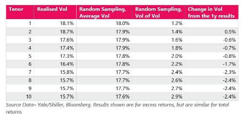
If annual returns are independent that suggests active mean reversion isn’t happening; however, it merits a deeper look. Another test is to compare annualized standard deviations – the idea being that any active reversion should result in lower volatilities for long-term holding periods.
However, because there is not that much data, we found the values obtained varied depending on the starting point. Particularly for the longer periods, the standard deviation of excess returns will be different if you take periods from (say) 1870-1880, 1880-1890, and so on, or if you take periods 1871-1881, 1881-1891, etc. To compensate, we took the average over each such “run”; that is, for ten year periods, we defined run 1 as: 1871-1880, 1881-1890…, and run 2 as: 1872-1882, 1882-1892… etc. We then took the average standard deviation over all the “runs” for each time period.
There is some risk reduction, but not much. For context, the 10y runs have volatilities ranging from 13% to 20%. There is even meaningful variation in the annual volatility depending on which month you start from.
These are relatively ambiguous results. Fortunately, we can test them. If there is an active pull to par, then the order of returns is relevant. If there isn’t, then it isn’t. So, if we sample the same distribution randomly, and repeat these calculations, we can see whether we could get the same results just by chance. To avoid complications around capturing the equity return distribution accurately, we just sample each year’s return with equal probability. We then do this for 10,000 simulated 146-year period, and record the averaged volatility of each tenor each time.
As expected, when sampling randomly, there’s no meaningful change in average volatility through time. However, we can also look at the volatility of these volatilities, to see if the realised values are distinctive. At no horizon is the realised volatility even one standard deviation away from the realised 1-year volatility.
So there’s reason to believe that returns are independent, but not much evidence for any form of active reversion. It might happen, but it’s hard to justify. Next time someone suggests “riding out the storm”, or “getting out at the peak”, it may be worth going back to the maths.
|


